Method Development Plots

Packages

We need to load the following packages.

library(tidyverse)
library(ggplot2)
library(readxl)
library(stringr)
#If you dont already have these loaded. Use install.packages("packagename") in the console. 

Sorbent Mass Optimization

First step is to read the datasheets and create a dataset.

#Ethyl Acetate
SMO_EA <-read_excel("Experimental_run_theresa.xlsx", sheet =4)
#Split in to Geosmin and MIB so we can add the "type". 
geosmin <-SMO_EA[,c(1:3)]
colnames(geosmin)<-c("Sorbent Mass", "Val", "SD")
geosmin$type<-c(rep("Geosmin", 3))

MIB <-SMO_EA[,c(1,4:5)]
colnames(MIB)<-c("Sorbent Mass", "Val", "SD")
MIB$type<-c(rep("2-MIB", 3))

# Bind geosmin and MIB
SMO_EA<-rbind(geosmin, MIB)
#Add column that indicates the eluent
SMO_EA$eluent <- c(rep( "Ethyl Acetate", 6))

# Repeat With Toluene
SMO_TL <-read_excel("Experimental_run_theresa.xlsx", sheet =5)
geosmin <-SMO_TL[,c(1:3)]
colnames(geosmin)<-c("Sorbent Mass", "Val", "SD")
geosmin$type<-c(rep("Geosmin", 3))

MIB <-SMO_TL[,c(1,4:5)]
colnames(MIB)<-c("Sorbent Mass", "Val", "SD")
MIB$type<-c(rep("2-MIB", 3))
SMO_TL<-rbind(geosmin, MIB)
SMO_TL$eluent <-c(rep("Toluene", 6))

# Combine Toluene and Ethyl Acetate 
SMO <- rbind(SMO_EA, SMO_TL)

## Remove mg and reset levels

SMO$`Sorbent Mass`<-str_remove_all(SMO$`Sorbent Mass`, "mg")
SMO$`Sorbent Mass`<-as.factor(SMO$`Sorbent Mass`)
SMO$`Sorbent Mass`<-ordered(SMO$`Sorbent Mass`, levels = c("500", "1000", "1500"))

Now we are ready to make the plots

## Scatter Plot
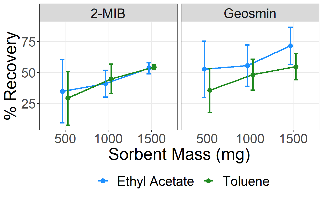
ggplot(SMO)+geom_point(aes(x = `Sorbent Mass`, y = Val, col = eluent),  position = position_dodge(width =0.25),
                       size = 3)+
  ylab("% Recovery") + theme_bw() + scale_color_manual(values = c("dodgerblue", "forestgreen"))+
  theme(text = element_text(size = 24),
        legend.position = "bottom")+guides(fill = guide_legend(""))+
  geom_line(aes(x = `Sorbent Mass`, y = Val, col = eluent, group = eluent),  position = position_dodge(width =0.25),
                       size = 1)+

  geom_errorbar(aes(x = `Sorbent Mass`, ymin = Val - SD, ymax = Val+SD, col = eluent), position = position_dodge(width =0.25),
               width = 0.2, size =1)+
  guides(color = guide_legend(""))+facet_wrap(~type)+xlab("Sorbent Mass (mg)")

### Column Plot

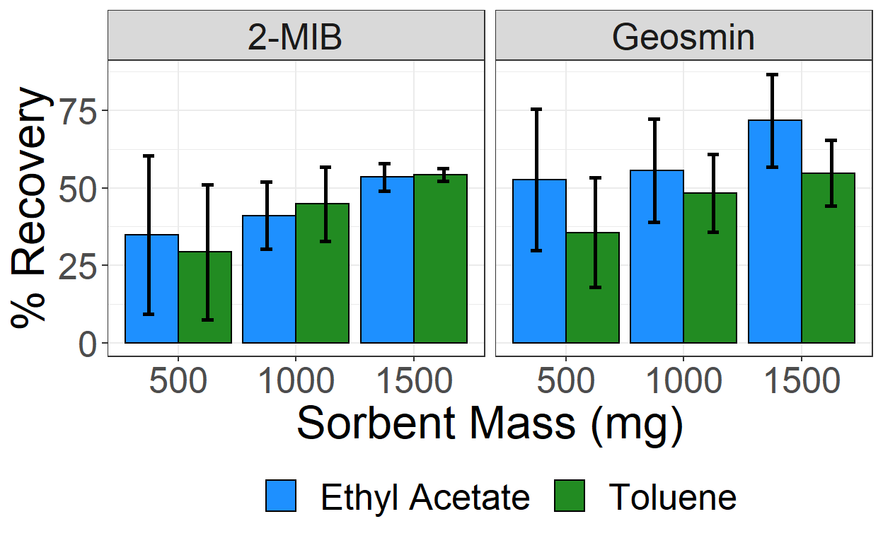
ggplot(SMO)+geom_col(aes(x = `Sorbent Mass`, y = Val, fill = eluent),  position = "dodge",
                       col = "black")+
  ylab("% Recovery") + theme_bw() + scale_fill_manual(values = c("dodgerblue", "forestgreen"))+
  theme(text = element_text(size = 24),
        legend.position = "bottom")+guides(fill = guide_legend(""))+

  geom_errorbar(aes(x = `Sorbent Mass`, ymin = Val - SD, ymax = Val+SD, col =eluent), position = position_dodge(width =1),
               width = 0.2, size =1, show.legend = F)+scale_color_manual(values = c("black", "black"))+
  guides(color = guide_legend(""))+facet_wrap(~type)+xlab("Sorbent Mass (mg)")

Elution Shaking Times

Make a dataset

#Read and create set
EST <-read_excel("Experimental_run_theresa.xlsx", sheet =7)
geosmin <-EST[,c(1:3)]
colnames(geosmin)<-c("Shaking Time", "Val", "SD")
geosmin$type<-c(rep("Geosmin", 3))

MIB <-EST[,c(1,4:5)]
colnames(MIB)<-c("Shaking Time", "Val", "SD")
MIB$type<-c(rep("2-MIB", 3))
EST<-rbind(geosmin, MIB)

Now we can make plots

#Scatter Plot
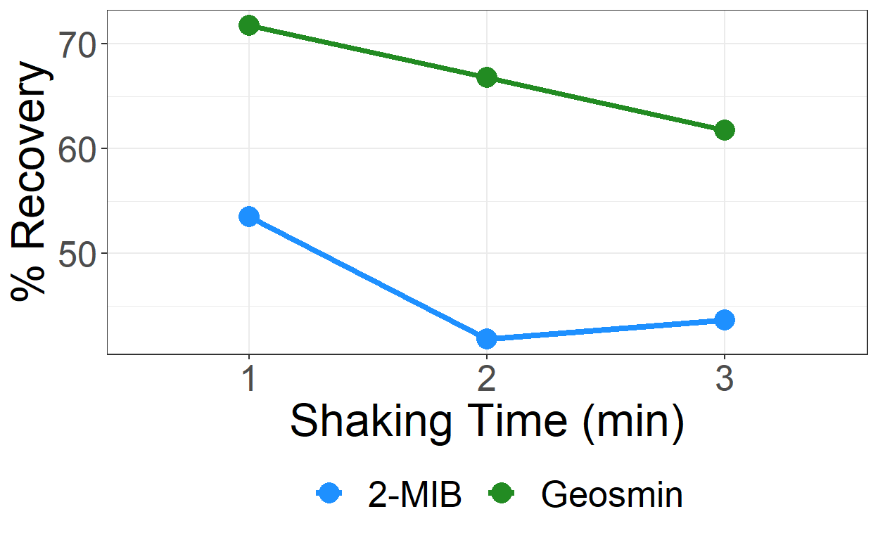
ggplot(EST)+geom_point(aes(x = as.factor(`Shaking Time`), y = Val, col =type),  
                       size =5)+
  ylab("% Recovery") + theme_bw() + 
  theme(text = element_text(size = 24),
        legend.position = "bottom")+guides(fill = guide_legend(""))+
  geom_line(aes(x = as.factor(`Shaking Time`), y = Val, col =type, group = type), size = 1.5)+

  guides(color = guide_legend(""))+xlab("Shaking Time (min)")+ scale_color_manual(values = c("dodgerblue", "forestgreen"))

#Column Plot
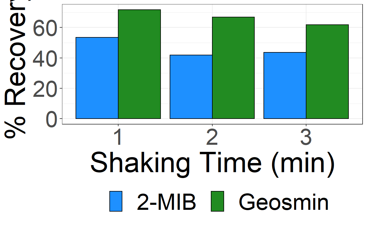
ggplot(EST)+geom_col(aes(x = as.factor(`Shaking Time`), y = Val, fill =type),  position = "dodge",col ="black")+
  ylab("% Recovery") + theme_bw() + 
  theme(text = element_text(size = 36),
        legend.position = "bottom")+guides(fill = guide_legend(""))+
  
  guides(color = guide_legend(""))+xlab("Shaking Time (min)")+ scale_fill_manual(values = c("dodgerblue", "forestgreen"))

Sorbent Selection

Make a dataset

#Read and create set
SS <-read_excel("Experimental_run_theresa.xlsx", sheet =1)
geosmin <-SS[,c(1:3)]
colnames(geosmin)<-c("Material", "Val", "SD")
geosmin$type<-c(rep("Geosmin", 3))

MIB <-SS[,c(1,4:5)]
colnames(MIB)<-c("Material", "Val", "SD")
MIB$type<-c(rep("2-MIB", 3))
SS<-rbind(geosmin, MIB)

Now we can make plots

#Scatter Plot
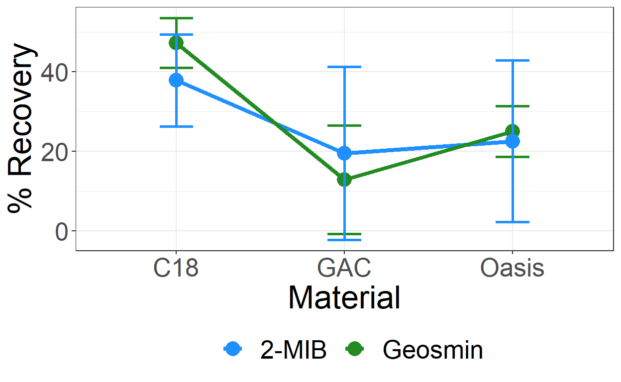
ggplot(SS)+geom_point(aes(x = as.factor(`Material`), y = Val, col =type),  
                       size =5)+
  ylab("% Recovery") + theme_bw() + 
  theme(text = element_text(size = 24),
        legend.position = "bottom")+guides(fill = guide_legend(""))+
  geom_line(aes(x = as.factor(`Material`), y = Val, col =type, group = type), size = 1.5)+
    geom_errorbar(aes(x = `Material`, ymin = Val - SD, ymax = Val+SD, col =type),
               width = 0.2, size =1, show.legend = F)+

  guides(color = guide_legend(""))+xlab("Material")+ scale_color_manual(values = c("dodgerblue", "forestgreen"))

#Column Plot
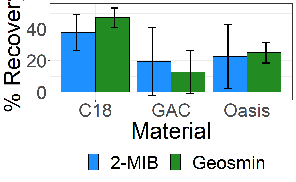
ggplot(SS)+geom_col(aes(x = as.factor(`Material`), y = Val, fill =type),  position = "dodge",col ="black")+
  ylab("% Recovery") + theme_bw() + 
  theme(text = element_text(size = 36),
        legend.position = "bottom")+guides(fill = guide_legend(""))+
    geom_errorbar(aes(x = `Material`, ymin = Val - SD, ymax = Val+SD, col =type), position = position_dodge(width =1),
               width = 0.2, size =1, show.legend = F)+scale_color_manual(values = c("black", "black"))+
  
  guides(color = guide_legend(""))+xlab("Material")+ scale_fill_manual(values = c("dodgerblue", "forestgreen"))

Solvent Selection

Make a dataset

#Read and create set
SS2 <-read_excel("Experimental_run_theresa.xlsx", sheet =2)
geosmin <-SS2[,c(1:3)]
colnames(geosmin)<-c("Solvent", "Val", "SD")
geosmin$type<-c(rep("Geosmin", 3))

MIB <-SS2[,c(1,4:5)]
colnames(MIB)<-c("Solvent", "Val", "SD")
MIB$type<-c(rep("2-MIB", 3))
SS2<-rbind(geosmin, MIB)

Now we can make plots

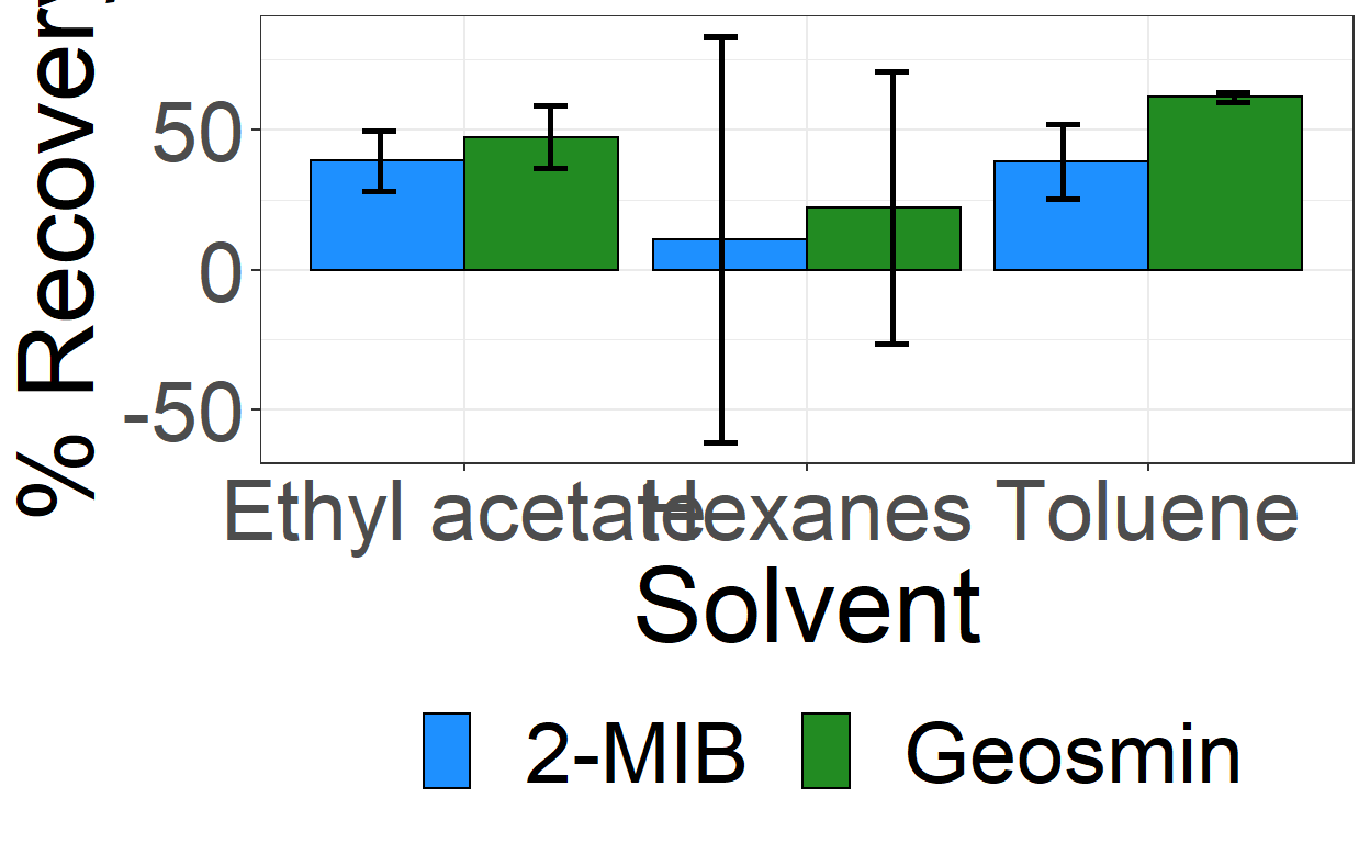
#Scatter Plot
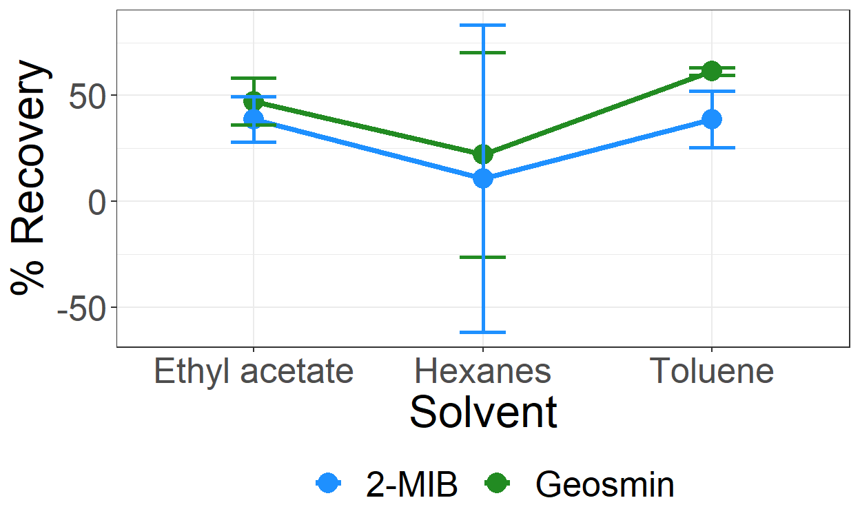
ggplot(SS2)+geom_point(aes(x = as.factor(`Solvent`), y = Val, col =type),  
                       size =5)+
  ylab("% Recovery") + theme_bw() + 
  theme(text = element_text(size = 24),
        legend.position = "bottom")+guides(fill = guide_legend(""))+
  geom_line(aes(x = as.factor(`Solvent`), y = Val, col =type, group = type), size = 1.5)+
    geom_errorbar(aes(x = `Solvent`, ymin = Val - SD, ymax = Val+SD, col =type),
               width = 0.2, size =1, show.legend = F)+

  guides(color = guide_legend(""))+xlab("Solvent")+ scale_color_manual(values = c("dodgerblue", "forestgreen"))

#Column Plot
ggplot(SS2)+geom_col(aes(x = as.factor(`Solvent`), y = Val, fill =type),  position = "dodge",col ="black")+
  ylab("% Recovery") + theme_bw() + 
  theme(text = element_text(size = 36),
        legend.position = "bottom")+guides(fill = guide_legend(""))+
    geom_errorbar(aes(x = `Solvent`, ymin = Val - SD, ymax = Val+SD, col =type), position = position_dodge(width =1),
               width = 0.2, size =1, show.legend = F)+scale_color_manual(values = c("black", "black"))+
  
  guides(color = guide_legend(""))+xlab("Solvent")+ scale_fill_manual(values = c("dodgerblue", "forestgreen"))